Does R square Measure the Predictive Capacity or Statistical Sufficiency ?
The way that R-squared shouldn’t be utilized for choosing if you have a satisfactory model is illogical and is once in a while clarified unmistakably. This exhibit diagrams how R-squared integrity of-fit functions in relapse investigation and relationships while demonstrating why it’s anything but a proportion of measurable sufficiency, so ought not to propose anything about future prescient execution.
The R-squared Goodness-of-Fit measure is one of the most broadly accessible insights going with the yield of relapse investigation in factual programming. Maybe incompletely because of its far-reaching accessibility, it is additionally one of the frequently misjudged ones.
Initial, a concise update on R-squared (R2). In a relapse with a solitary free factor, R2 is determined as the proportion between the variety clarified by the model and the all-out watched variety. It is regularly called the coefficient of assurance and can be deciphered as the extent of variety clarified by the presented indicator. In such a case, it is proportionate to the square of the convection coefficient of the watched and fitted estimations of the variable. In various relapse, it is known as the coefficient of different assurance and is regularly determined utilizing a modification that punishes it is worth relying upon the number of indicators utilized.
In neither of these cases, be that as it may, does R2 measure whether the correct model was picked, and therefore, it doesn’t quantify the prescient limit of the acquired fit. This is accurately noted in numerous sources, yet not many clarify that factual sufficiency is essential for effectively deciphering a coefficient of assurance. Special cases incorporate Spanos 2019 [1] wherein one can peruse “underscore that the above measurements [R-squared and others] are significant just for the situation where the evaluated straight relapse model is factually sufficient,” and Hagquist and Stenbeck (1998).[2] It is much rarer to see instances of why that is the situation with an exemption being Ford 2015.[3]
The current article incorporates a more extensive arrangement of models that explain the job and constraints of the coefficient of assurance. To keep it reasonable, just a single variable relapse is analyzed. The Appeal of R-squared
First, let us examine the utility of R2 and to see why it is so easy to incorrectly interpret it as a measure of statistical adequacy and predictive accuracy when it is neither. Using a comparison with the simple linear correlation coefficient will help us understand why it behaves the way it does.
Figure 1 below is based on extracted data from 32 price offers for second-hand cars of one high-end model. The idea is to examine the relationship between car age (x-axis) and price (y-axis, in my local currency unit).
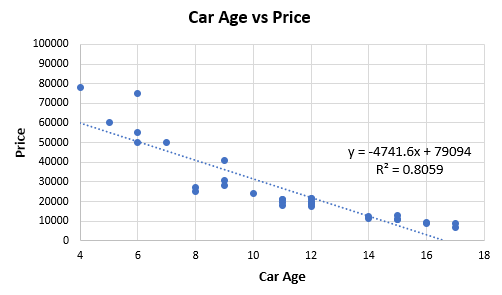
Entering the information into a connection coefficient adding machine, we acquire a Pearson’s r of — 0.8978 (p-esteem 0 to the eighth decimal spot, 95%CI: — 0.9493, — 0.7992). These outcomes in an agreeable R2 of 0.8059, which would, truth be told, be viewed as high by numerous guidelines. The connection figuring is comparable to running a straight relapse. Eyeballing the fit makes it clear that it can probably be improved by picking a non-straight relationship from the exponential family all things considered:

The fit acquired with the relapse condition that appeared in Figure 2 above has an R2 estimation of 0.9465, this one is constrained to supplant the straight with the exponential model. As the exponential model clarifies a greater amount of the difference, one may think it is a superior portrayal of the hidden information creating an instrument, and maybe this likewise implies it will have better prescient exactness. That is the natural intrigue of utilizing R-squared to pick between one model and another. Notwithstanding, this isn’t really so as the following parts will illustrate.
Different Underlying Model, Same R-squared?
Imagine a scenario in which disclosed to you that you can get the equivalent R2 measurement for a direct relapse of two particular datasets while realizing that the fundamental model is very extraordinary in each set. This can be shown by a straightforward reenactment. The accompanying R code produces indicator and reaction esteems dependent on two separate genuine models — one is direct, and the other is exponential:
set.seed(1);                           # set seed for replicability
x <- seq(1,10,length.out = 1000)       # predictor values
y <- 1 + 1.5*x + rnorm(1000, 0, 0.80)  # response values produced as a linear function of x and random noise with sd of 0.649
summary(lm(y ~ x))$r.squared           # print R-squared for the linear model
y <- x^2 + rnorm(1000, 0, 0.80)        # response values produced as an exponential function of x and random noise with sd of 1.377
summary(lm(y ~ x))$r.squared           # print R-squared for the exponential model
The consequence of the straight model fit is R2 = 0.957 for both. In any case, we realize that one lot of information originates from a direct reliance and another from an exponential one. This can be additionally investigated utilizing the plots of the reaction variable y, as appeared in Figure 3.
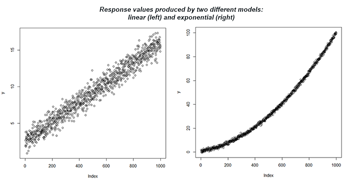
On the off chance that one uses an R-squared edge to acknowledge a model, they would probably acknowledge a straight model for the two conditions. In spite of a similar R-squared measurement created, the prescient legitimacy would be somewhat extraordinary relying upon what the genuine reliance is. In the event that it is really direct, at that point the prescient exactness would be very acceptable. Else, it will be a lot more unfortunate. In this sense, R-Squared is certainly not a decent proportion of prescient mistake. The standard blunder would have been a vastly improved guide being about multiple times littler in the principal case.
Low R-squared Doesn’t Necessarily Mean an Inadequate Statistical Model
In the principal model, the standard deviation of the irregular commotion was kept the equivalent, and we changed just the kind of reliance. In any case, the coefficient of assurance is fundamentally impacted by the scattering of the arbitrary mistake term, and this is the thing that we will look at straightaway. The code beneath produces mimicked R2 values for various degrees of the standard deviation of the blunder term for y while keeping the kind of reliance the equivalent. The information is produced with a satisfactory model for the blunder term, and the relationship is straight. It fulfills the straightforward relapse model on all records: ordinariness, zero mean, homoskedasticity, no autocorrelation, and no collinearity as only a solitary variable is included.
r2 <- function(sd){
  x <- seq(1,10,length.out = 1000)       # predictor values
  y <- 2 + 1.2*x + rnorm(1000,0,sd = sd) # response values produced as a linear function of x and random noise with sd of sd
  summary(lm(y ~ x))$r.squared           # print R-squared
}
sds <- seq(0.5,40,length.out = 40) # generate sd values with a step of 0.5
res <- sapply(sds, r2) # calculate the function with each sd value
plot(res ~ sds, type="b", main="R-squared for different values of Sigma", xlab="Sigma (Standard Deviation)", ylab="Average R-squared")
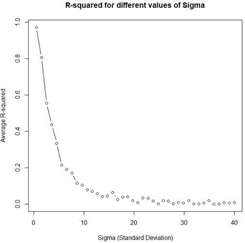
Despite the fact that the measurable model fulfills all prerequisites and is in this manner very much indicated, with expanding change in the blunder term, the R2 esteem will in general zero. The above is an exhibit of why it can’t be utilized as a proportion of measurable insufficiency.
High R-squared Doesn’t Necessarily Mean an Adequate Statistical Model
Something contrary to the above situation can occur if the model is miss-indicated at this point the standard deviation is adequately little. This will in general produce high R2 values as shown by running the code beneath.
r2 <- function(sd){
  x <- seq(1,10,length.out = 1000)       # predictor values
  y <- x^2 + rnorm(1000,0,sd = sd)       # response values produced as a linear function of x and random noise with sd of sd
  summary(lm(y ~ x))$r.squared           # print R-squared
}
sds <- seq(0.5,40,length.out = 40) # genearte sd values with a step of 0.5
res <- sapply(sds, r2) # calculate the function with each sd value
plot(res ~ sds, type="b", main="R-squared for different values of Sigma", xlab="Sigma (Standard Deviation)", ylab="Average R-squared")
It should produce a plot like the one shown in Figure 5.
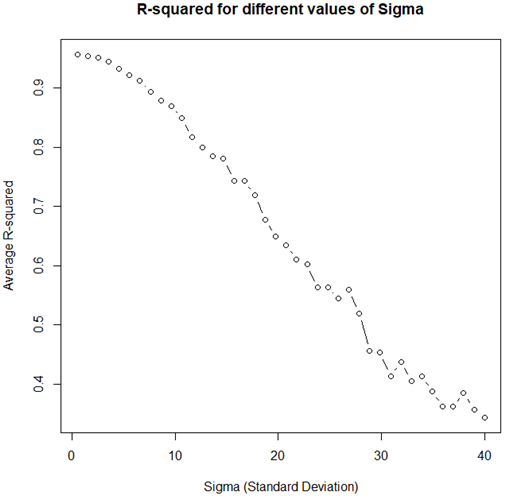
As clear, even with an unequivocally non-straight basic model, high R-squared qualities can be watched for a wide scope of sigma esteems. This implies even self-assertively high estimations of the measurement can’t really be taken as proof for model ampleness.
conclusion
Ideally, the above models fill in as an adequate outline of the threats of over-deciphering the coefficient of assurance. While it is a proportion of decency of-fit, it possibly increases meaning if the model is satisfactory as for the fundamental instrument producing the information. Utilizing it as a proportion of model ampleness isn’t justified, and to the degree to which homing in on the right model effects or prescient mistake, it’s anything but a proportion of it either. Regardless of whether that leaves any valuable spot for it at all is as yet a matter of discussion.
References:
[1] Spanos A. (2019). “Probability Theory and Statistical Inference: Empirical Modeling with Observational Data.” Cambridge University Press. p.635
[2] Hagquist, C., Stenbeck, M. (1998) “Goodness of Fit in Regression Analysis — R 2 and G 2 Reconsidered.” Quality and Quantity. 32, pp.229–245
[3] Ford C. (2015). “Is R-squared Useless? https://data.library.virginia.edu/is-r-squared-useless/
Bio: Arpit Bhushan Sharma (B.Tech, 2016–2020) Electrical & Electronics Engineering, KIET Group of Institutions Ghaziabad, Uttar Pradesh, India. | Project Manager — Project4jungle | Chief Organising Officer — Waco | Project Manager— Edusmith | Student Member R10 IEEE | Student Member PES | Voice: +91 8445726929 | E-mail: bhushansharmaarpit@gmail.com


Comments
Post a Comment